
tldr: DCT compression methods can introduce visible artifacts at block boundaries of images. In this post we take a look at an algorithm proposed by Luo and Ward [1] for the removal of edges of the blocks in regions that are affected by blockiness effects. The algorithm uses an adaptive approach where it considers the local information of the image before proceeding with the modification of pixel values based on weighted average of neighbouring blocks. Experiments show that the algorithm can significantly reduce the visible blockiness artifacts from the given images.
Data compression is the process of removing the redundant data present in a given image while trying to preserve as much information present in the original image as possible. The common types of data redundancies can be characterized into three categories.
1) Coding Redundancy
2) Spatial Redundancy
3) Irrelevant Information.
Several methods are available compress the given image for transmission and storage. However these methods come with their own set of challenges. For example block-based DCT compression methods can introduce certain types of visible artifacts at block boundaries[4]. This digression is because of coarse quantization of coefficients. If we do not take into account the existing correlations among adjacent blocks then these types of “blocking artifact” can occur. Several filtering techniques exist to reduce the blockiness by reducing the high frequency components present near the block boundaries. In this work we will take a look at the technique proposed by Luo and Ward [1] for removing the blocking effects in smooth regions of the image.
The algorithm proposed by Luo and Ward is based on the idea that some of the DCT coefficients of a step function(representing a sharp edge) have nonzero values. First step in this approach is to detect the strong texture and edge regions based on frequency co-efficients. We iterate through the image and extract two neighboring 8x8 blocks in each step. If they have similar frequency properties and the boundary 8x8 pixel contains no high frequencies then portion of image is considered to be smooth. DCT filtering has shown to be effective in this case as it ensures pixel value continuity.
Our core algorithm consists of following steps:
Extracting adjacent blocks

Figure 1. Blockiness Diagram [4]
We pick two blocks A and B from the given image as show in figure 1. Block C will contain boundary pixels as it will contains right and left half of Block A and Block B respectively. In the first phase we pick horizontally adjacent blocks and iterate column wise through the image, while in the second phase we pick vertically adjacent blocks while iterating row wise through the image.
ii. Calculating DCT transform
The Next step will be to calculate the DCT matrix of all the three blocks. DCT has the ability to concentrate information and is used in image compression applications. The definition of the two-dimensional DCT for an input image A and output image B is:
$B_{p q}=\alpha_{p} \alpha_{q} \sum_{m=0}^{M-1} \sum_{n=0}^{N-1} A_{m n} \cos \frac{\pi(2 m+1) p}{2 M} \cos \frac{\pi(2 n+1) q}{2 N}, \begin{aligned}&0 \leq p \leq M-1 \&0 \leq q \leq N-1\end{aligned}$
where
$$\alpha_{p}=\left{\begin{array}{l}
\frac{1}{\sqrt{M}}, p=0 \
\sqrt{\frac{2}{M}}, 1 \leq p \leq M-1
\end{array}\right.$$
and
$$
\alpha_{q}= \begin{cases}\frac{1}{\sqrt{N}}, & q=0 \ \sqrt{\frac{2}{N}}, & 1 \leq \mathrm{q} \leq \mathrm{N}-1\end{cases}
$$
Threshold Comparisons:
To adapt the filtering to the local information content of the image we apply the following conditions. They will ensure that modifications are done to relatively smooth regions.
where values for T1, T2, T3 are predefined and are found through experimentation. If the above three conditions are met we can proceed with blockiness reduction in DCT domain as explained in next step 4.
a. $\left|F_{a}(0,0)-F_{b}(0,0)\right|<T_{1}$
b. $\left|F_{a}(0,1)-F_{b}(0,1)\right|<T_{2}$.
c. $\left|F_{c}(3,3)\right|<T_{3}$.
where values for T1, T2, T3 are predefined and are found through experimentation. If the above three conditions are met we can proceed with blockiness reduction in DCT domain as explained in next step 4.
iv. Computing Modified Block C
It is observed that Block C will have non-zero values at row 0 and column= 0,1,3,5,7 of the image. Hence we will modify five coefficients values of block C, but we have to modify them in a way that original information (e.g sharp edges) in the image should not be lost during the process. Modified block C can be computed using weighted average of blocks A, B, and C which makes filtering more adaptive to image contents. Following equations are used for the computing the modified block C which takes into account information present in neighboring blocks B and C.
$$
F_{M c}(0, v)=\alpha_{0} F_{c}(0, v)+\beta_{0}\left[F_{a}(0, v)+F_{b}(0, v)\right]
$$
where
$$
\begin{aligned}
v &=0,1 \
F_{M c}(0, v) &=\alpha_{1} F_{c}(0, v)+\beta_{1}\left[F_{a}(0, v)+F_{b}(0, v)\right]
\end{aligned}
$$
where
$$
\begin{aligned}
v &=3,5,7 \
F_{M c}(u, v) &=F_{c}(u, v) \quad \text { for all } \quad v \neq 0,1,3,5,7
\end{aligned}
$$
i. Replacing input image with inverse DCT of Modified C block
In this step we compute the inverse DCT of modified block C and replace the original block C pixel values with the newly computed values. The new modified pixel values of block C can be represented by the following equation:
$$
C_{M c}(k, l)=c(k, l)+\xi(l)
$$
$\begin{aligned} C_{M c}(k, l)=& c(k, l)+\xi(l) \ \text { where } \ \xi(l)=& \sum_{u=0}^{N-1} \sum_{v=0}^{N-1}\left(C_{u} C_{v}\left(F_{M c}(u, v)-F_{c}(u, v)\right)\right.\=&\left.\times W_{D C T}(u, k) W_{D C T}(v, l)\right) \=& C_{0} C_{0}\left[F_{M c}(0,0)-F_{c}(0,0)\right] \ &+\sum_{i=0}^{3} C_{0} C_{v}\left[F_{M c}(0, v)-F_{c}(0, v)\right] \ & \times W_{D C T}(v, l) \end{aligned}$
where $v=2 i+1$.
Steps i to v will remove discontinuity present at boundary pixels of horizontally adjacent blocks. These step are repeated in Phase II to remove discontinuity from vertically adjacent blocks.
Coding Listing:
%read given compressed image image
f = imread('portrait_compressed_10.jpg');
input = f;
ref = imread('portrait.bmp');
f = double(f);
img_size = size(f);
%Declare Thresholds
Threshold_1 = 350;
Threshold_2 = 120;
Threshold_3 = 60;
%----------------------------------------------------------
%PHASE 1: iterating through input image using Horizontally Adjacent Blocks
%----------------------------------------------------------
for row_pixel = 1:8:(img_size(1) - 16)
for column_pixel = 1:8:(img_size(2) - 16)
% Extract 8x8 Blocks A,B,C. Blocks C is an overlap of Block A and B
% and contains boundry pixels of both blocks.
f_blockA = f(row_pixel:row_pixel + 7,column_pixel: column_pixel + 7);
f_blockC = f(row_pixel:row_pixel+7,column_pixel + 4 : column_pixel + 11);
f_blockB = f(row_pixel :row_pixel +7,column_pixel + 8: column_pixel + 15);
%calculate two-dimensional discrete cosine transform of Blocks A,B,C
DCT_blockA = dct2(f_blockA);
DCT_blockB = dct2(f_blockB);
DCT_blockC = dct2(f_blockC);
%Condition 1: checks if Block A has a similar horizontal frequency property as block B.
%in the if condition we check if first row of the DCT matrix block A
%and of block B are close in values or not
%Condition 2: boundary between block A and block B belongs to a relatively smooth region.
% we check if block C is of low frequency content. if textures and other strong diagonal edges are present then it
% would result in relatively high values of DCT co-efficients
diff1 = (DCT_blockA(1,1) - DCT_blockB(1,1));
diff2 = (DCT_blockA(1,2) - DCT_blockB(1,2));
diff3 = (DCT_blockC(4,4));
if (diff1 < Threshold_1 && diff2 < Threshold_2 && diff3 < Threshold_3)
%calculating the modified DCT coefficient of block C.
%New values for column 0,1,3,5,7 would be calculated using weighted average of blocks A,B,C
%alpha = 0.6, Beta = 0.2 for case v=0, v=1.
%case v=0
DCT_blockC(1,1) = 0.6 * DCT_blockC(1,1) + 0.2 * (DCT_blockA(1,1) + DCT_blockB(1,1));
%case v=1
DCT_blockC(1,2) = 0.6 * DCT_blockC(1,2) + 0.2 * (DCT_blockA(1,2) + DCT_blockB(1,2));
%0.5 and 0.25 are the values of alpha and beta are used for columns 3,5,7
%case v=3
DCT_blockC(1,4) = 0.5 * DCT_blockC(1,4) + 0.25 * (DCT_blockA(1,4) + DCT_blockB(1,4));
%case v=5
DCT_blockC(1,6) = 0.5 * DCT_blockC(1,6) + 0.25 * (DCT_blockA(1,6) + DCT_blockB(1,6));
%calculate inverse dct of modified block C
%case v=7
DCT_blockC(1,8) = 0.5 * DCT_blockC(1,8) + 0.25 * (DCT_blockA(1,8) + DCT_blockB(1,8));
%calculate inverse dct
inv_DCT_blockC = idct2(DCT_blockC);
%replace f_blockC with inverse dct of modified block C
f(row_pixel : row_pixel + 7,column_pixel + 4: column_pixel + 11) = inv_DCT_blockC(:,:);
end
end
end
%----------------------------------------------------------
%PHASE 2: iterating through image using Vertically Adjacent Blocks
%----------------------------------------------------------
for column_pixel2 = 1:8:(img_size(2) - 16)
for row_pixel2 = 1:8:(img_size(1) - 16)
% Extract 8x8 Blocks A,B,C. Blocks C is an overlap of Block A and B
% and contains boundry pixels of both blocks.
f_blockA = f(row_pixel2:row_pixel2 + 7,column_pixel2: column_pixel2 + 7);
f_blockC = f(row_pixel2 + 4:row_pixel2 + 11,column_pixel2 : column_pixel2 + 7);
f_blockB = f(row_pixel2 + 8 :row_pixel2 +15,column_pixel2: column_pixel2 + 7);
%calculate two-dimensional discrete cosine transform of Blocks A,B,C
DCT_blockA = dct2(f_blockA);
DCT_blockB = dct2(f_blockB);
DCT_blockC = dct2(f_blockC);
%Condition 1: checks if Block A has a similar horizontal frequency property as block B.
%in the if condition we check if first row of the DCT matrix block A
%and of block B are close in values or not
%Condition 2: boundary between block A and block B belongs to a relatively smooth region.
% we check if block C is of low frequency content. if textures and other strong diagonal edges are present then it
% would result in relatively high values of DCT co-efficients
diff1 = (DCT_blockA(1,1) - DCT_blockB(1,1));
diff2 = (DCT_blockA(2,1) - DCT_blockB(2,1));
diff3 = (DCT_blockC(4,4));
if (diff1 < Threshold_1 && diff2 < Threshold_2 && diff3 < Threshold_3)
%calculating the modified DCT coefficient of block C.
%New values for column 0,1,3,5,7 would be calculated using weighted average of blocks A,B,C
%alpha = 0.6, Beta = 0.2 for case v=0, v=1.
%case v=0
DCT_blockC(1,1) = 0.6 * DCT_blockC(1,1) + 0.2 * ( DCT_blockA(1,1) + DCT_blockB(1,1));
%case v=1
DCT_blockC(2,1) = 0.6 * DCT_blockC(2,1) + 0.2 * (DCT_blockA(2,1) + DCT_blockB(2,1));
%0.5 and 0.25 are the values of alpha and beta are used for columns 3,5,7
%case v=3
DCT_blockC(4,1) = 0.5 * DCT_blockC(4,1) + 0.25 * (DCT_blockA(4,1) + DCT_blockB(4,1));
%case v=5
DCT_blockC(6,1) = 0.5 * DCT_blockC(6,1) + 0.25 * (DCT_blockA(6,1) + DCT_blockB(6,1));
%case v=7
DCT_blockC(8,1) = 0.5 * DCT_blockC(8,1) + 0.25 * (DCT_blockA(8,1) + DCT_blockB(8,1));
%calculate inverse dct of modified block C
inv_DCT_blockC = idct2(DCT_blockC);
%replace the corresponding original image pixels with inverse dct of modified block C
f(row_pixel2 + 4:row_pixel2 + 11,column_pixel2 : column_pixel2 + 7) = inv_DCT_blockC(:,:);
end
end
end
%----------------------------------------------------------
%Display and Compare input/output images
%----------------------------------------------------------
subplot(1,2,1), imshow(input), title('Original image')
subplot(1,2,2), imshow(uint8(f)), title('Filtered image')
%----------------------------------------------------------
%Calculate PeakSNR values
%----------------------------------------------------------
[peaksnr, snr] = psnr(uint8(f), ref);
fprintf('\n The Peak-SNR value is %0.4f', peaksnr);
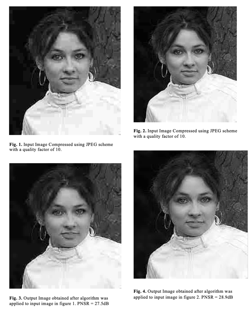
fprintf('\n The SNR value is %0.4f \n', snr);The following page(Figures 1-4) contains the input output visual comparisons of the images.
Future Improvements
Through our experiments I propose following future improvements in the code:
Adaptive Threshold values
Current Algorithm uses hard-coded threshold values to ensure original contents of the image remain preserved. Our aim here is to only remove sharp edges introduced by the compression algorithm and not remove any actual edges present in the image. The hard- coded values currently being used in the image can work well for some of the images but cannot generalize well. Therefore for our algorithm to work equally well with all sets of input images, we need to come up with a generic approach that uses local information of the image to come up with these values. The values should also be dependent of the bit rate of the given input image as they can result in varying amount of filtering for different bit rates.
Boundary Block value comparisons:
To save computations, only one pixel value comparison was done of the boundary containing block(condition 3 in step 3 of our algorithm). This step was to ensure that boundary containing block is of low frequency content[4]. Through experimentation I found that more number of comparisons can potentially result in better performance. However the correlation of computational savings vs quality gain is not clear at this point and further experimentation is needed to explore this.
[1] Ying Luo and Rabab K. Ward, “Removing the Blocking Artifacts of Block-Based DCT Compressed Images”, IEEE transactions on image processing, vol. 12, no. 7, July 2003.