
Deep Neural Networks (DNNs) are neural networks with architecture consisting of multiple layers of perceptrons, designed to solve complex learning problems. Deep Neural Networks focus on the need to process and classify complex, high-dimensional data, requiring the use of a large number of neurons in numerous layers. In these networks, each layer is fully connected to its adjacent layers.
In this post we take a look at the brief history of deep learning and Journey leading to its popularity.
A Deep Neural Network (DNN) is defined by Hinton et al. as “a feedforward artificial neural network that contains more than one hidden layer of hidden units”. DNN’s have a number of processing layers that can be used to learn representations of data with multiple tiers of abstraction. The different tiers are obtained by producing non-linear modules that are used to transform the representation at one tier into a representation at a more abstract tier. By using these tiers, features of the data used for classification is enhanced while irrelevant features are suppressed. Deep convolutional nets and recurrent nets are varieties of DNNs, and algorithms using them have brought about breakthroughs in processing text, images, video, speech and audio.
However as we'll see in this post it took a lot of effort to get here.
A major challenge at the inception of DNNs in the 1990s was the limited computational power of computers. DNNs faced challenges in terms of training and generalisation because they required a considerable number of training patterns to arrive at good solutions, which were hampered by the limited size of early labeled data sets. Moreover, traditional DNNs with large numbers of interconnections would overfit the data, and require different special training techniques to improve generalization. These issues led to the initial unpopularity of DNNs.
At this time, there were other competing models such as the Hidden Markov Model and the Support Vector Machine. Even though DNNs achieved similar or slightly better results (depending on the task) than the above models, they were much more difficult to train. Random initialisation did not yield good results and one had to be an expert and have sufficient domain knowledge in order to handcraft feature extractors. Furthermore, they lack the ability to train using unlabeled data, which is problematic as a lot of the real world data available to us is unlabeled.
For learning networks that had more than a few hidden layers, back-propagation alone did not work well in practice due to problems encountered such as the vanishing gradient and curse of dimensionality. The curse of dimensionality is the exponential increase in the number of possible combinations of input values as the number of input neurons increase. Without exponentially larger datasets to keep up, most of the possible combinations are zero, and the network faces training with sparse data. The learning time does not scale well with an increase in the total number of hidden layers. Other problems using backpropogation include overfitting the training set and the problem of local minima.
DNNs with many parameters are very powerful but are prone to overfitting. Overfitting generally occurs when the model is very complex and has too many input parameters compared to the outputs or observations, or a sparse data set. The model cannot generalise for new patterns because the trainable parameters adapt to the training set. One of the proposed solutions for overfitting is called ‘dropout’ and was suggested by Srivastava and others. The key idea of this technique is to randomly drop out units along with their connections, which prevents units from becoming excessively dependent.
It was shown by Hochreiter that algorithms relying on the calculation of a complete gradient tend to fade and eventually vanish while performing backpropogation. The gradients are calculated using the derivatives of the error function. From the chain rule of derivatives, the gradient becomes smaller in the lower layers and eventually becomes too small to make significant weight adjustments. One of the proposed solutions is a novel gradient-based method called the Long Short-Term Memory by Sepp Hochreiter and J¨urgen Schmidhuber that is capable of remembering error values for longer durations.
When the parameters were randomly initialized for gradient-based optimization methods such as the stochastic gradient descent, the DNN had a high possibility of ending up in a local minima. The network can lead to a poor local minimum if the parameters are not initialized sensibly, and this is more common as the depth of the network increases. Local minima are suboptimal solutions in the error space. In a deep network with many hidden layers, there are significant numbers of local minima. Unless the weights are already in the local area of the global minimum at the start of training, the result will likely fall into a suboptimal local minima.
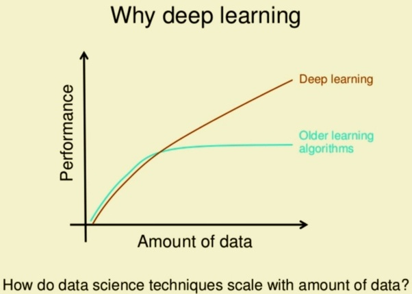
Despite initial unpopularity due to poor performance and small datasets, DNNs eventually came to wider use. There was an exponential growth of unlabeled datasets in the late 2000s. There was a need to use more unsupervised approaches, which was facilitated by Hinton and others when Deep Belief Networks (DBNs) were created. This was the first major breakthrough for DNNs. The key idea was to use ‘pre-training’ in order to learn features rather than having to handcraft them. This improvement made training DNNs much easier as features were learnt automatically.
Let's look understand how DBM are trained in a bit more detail:
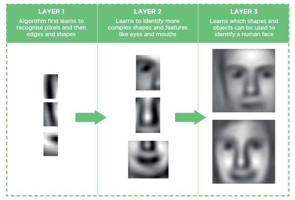
Deep Belief Networks: Deep Belief Networks (DBNs) is a stack of Restricted Boltzmann Machines (RBMs) and feature detectors. Training involves following a greedy, layerwise, unsupervised approach where each RBM receives pattern representations from the level below and learns to encode them in an unsupervised fashion. Conceptually these layers act as feature detectors and the network learns higher-level features (which represent more ‘abstract’ concepts found in the input) from the lower layers (which represent ‘low-level features’). High level abstract concepts are learned by building on simpler concepts that are learned by earlier layers at the beginning of the network. The training of DBNs is a two step process in which there is a pre-training phase and a fine-tuning phase. In pre-training the network is trained layer-by-layer greedily in an unsupervised fashion. When the network learns single layers, gradient ascent is used to get the optimum weight vector. Weights are updated using contrastive divergence and Gibbs-sampling.
In the RBM layer a vector is inputted to the visible units which are connected to the hidden layer. While going in the opposite direction the original input is reconstructed stochastically by finding the higher-order data correlations observed at the visible units. This process of going back and forth is repeated several times and is known as Gibbs sampling. Using this layer-wise training strategy helps in better initialization of the weights, thus solving the difficult optimization problem of deep networks.
Furthermore following the greedy layer wise approach, can provide good generalization because it initializes upper layers with better representations of relevant high level abstractions. After the pre-training step, the weights between every adjacent layers hold the values that represent the information present in the input data. But in order to get improved discriminative performance, the network is often fine-tuned according to supervised training criterion. This can be done by using gradient descent which uses the weightings learned in the previous pre-training phase. Overall it is observed that the learning algorithm proposed by Hinton and others. It has time complexity linear to the size and depth of the network, which allows us to train deep networks at a much faster rate compared to the old approaches.
Final major event was the advent of fast Graphic Processing Units that made it possible for networks to be trained more than ten times faster. A lot of the models created using DNNs started outperforming the other existing models. Another breakthrough was the use of convolution networks for the classification of the ImageNet database. With this rise in popularity it lead to DNNs being adopted in various domains such as computer vision and image processing, encouraging more researchers to explore DNNs and deep learning.
Deep Neural Networks and Images
Sometimes it was the innovation in architecture that solved a certain class of problems. e.g For images with even a modest number of pixels, DNNs do not scale well, and the full interconnectedness make DNNs computationally- and memory-intensive. This is because of the intractable numbers of connection weights to be trained. To process images of practical size while being computationally feasible, an alternative architecture was needed. And the answer came in the form of Convolutional Neural Networks (CNNs) which are a flavour of DNNs, structured with a reduced number of trainable weights. This results in a reduction in computing time and storage space, and a feasible solution to training with images of practical size.
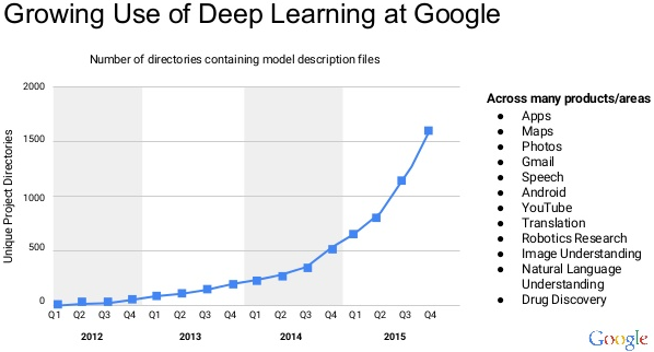
CNNs combined with ImageNet data trained on GPUs was the big bang moment in the history deep learning. Now almost all major product inside google use deep Learning.
References
Arel, I, Rose, D & Karnowski, T 2010, ‘Deep Machine Learning? A New Frontier in Artificial Intelligence Research [Research Frontier]’, IEEE Computational Intelligence Magazine, vol. 5, no. 4, p. 13, viewed 14 October 2015
Bengio, Y 2009, ‘Learning Deep Architectures for AI’, Foundations and TrendsR in Machine Learning, vol. 2, no. 1, pp. 1–127, viewed 3 October 2015,
Bengio, S & Bengio, Y 2000, ‘Taking on the Curse of Dimensionality in Joint Distributions Using Neural Networks’, IEEE Transactions on Neural Networks, vol. 11, no. 3, pp. 550- 557, viewed 3 October 2015,
Bengio, Y, Lamblin, P, Popovici, D & Larochelle, H 2007, ‘Greedy Layer-Wise Training of Deep Networks’, Advances In Neural Information Processing Systems 19, p. 153–158, viewed 4 October 2015,
Chapados, N & Bengio, Y 2001, ‘Input decay: Simple and Effective Soft Variable Selection’, Proceedings Of The International Joint Conference On Neural Networks, vol. 2, pp. 1233–1237, Washington DC, USA, viewed 16 October 2015
Farabet, C, Couprie, C, Najman, L & LeCun, Y 2013, ‘Learning Hierarchical Features for Scene Labeling’, IEEE Transactions On Pattern Analysis & Machine Intelligence, vol. 35, no. 8, pp. 1915–1929, viewed 6 October 2015, Computers & Applied Sciences Complete, EBSCO
Freeman, JA & Skapura, DM 1992, Neural Networks Algorithms, Applications, and Programming Techniques, Addison-Wesley Publishing Company, United States of America
Glorot, X & Bengio, Y 2010, ‘Understanding the Difficulty of Training Deep Feedforward Neural Networks’, Proceedings of the 13th International Conference on Arti- ficial Intelligence and Statistics (AISTATS), Sardinia, Italy, viewed 10 October 2015,
Hinton, G, Srivastava, N, Swersky, K, Tieleman, T & Mohamed, A n.d., ‘The ups and downs of backpropogation’, lecture notes, viewed 1 October 2015