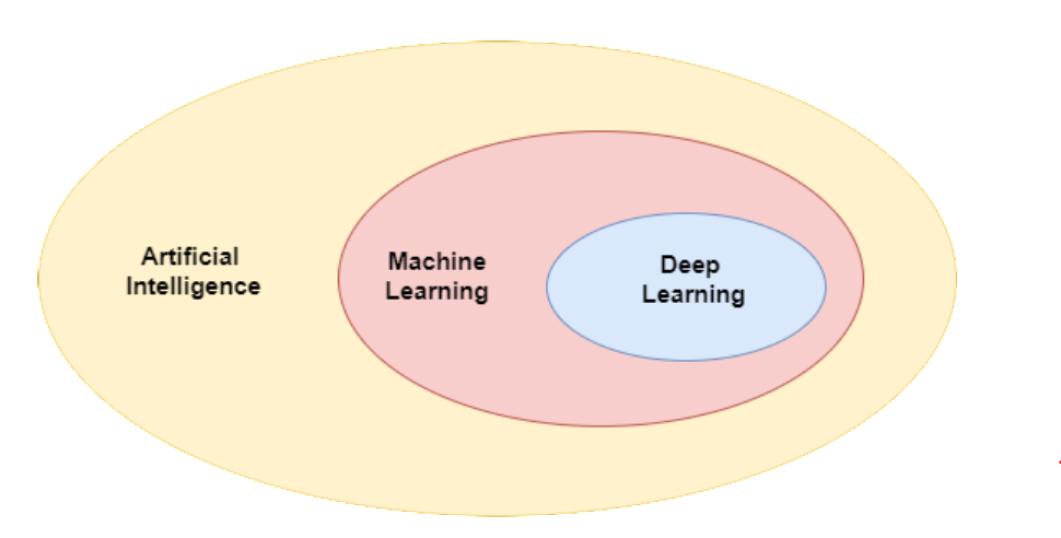
A long introduction to Machine Learning

Machine learning is closely related to Artificial intelligence

AI is about building machines or intelligent agents that exhibit intelligence.
ML enables machines to learn from experience, and is a sub-field of AI.
Deep learning focuses on a family of learning algorithms known as neural networks.

The focus of this series is on Machine Learning, so lets dig in:

Machine Learning uses a set of observations to uncover an underlying process. It enables us to tackle tasks that are too difficult to solve with fixed programs written and designed by human beings. In tackling machine learning we face some deep philosophical questions. Questions like, “What does it mean to learn?” and, “Can a computer learn?” and, “How do you define simplicity?” and, “Why does Occam’s Razor work? (Why do simple hypotheses do well at modeling reality?)” In a very deep sense, learning theorists take these philosophical questions — or at least aspects of them — give them fleshy mathematical bodies, and then answer them with theorems and proof.

A machine learning algorithm is an algorithm that is able to learn from data.

Formally, a reasonable definition of ML is as follows:

A computer program is said to learn from experience E with respect to some class of tasks T and performance measure P, if its performance at tasks in T, as measured by P, improves with experience E

Considering the above definition, from a task perspective we typically categorise machine learning as supervised, unsupervised, and reinforcement learning. In supervised learning, the training dataset includes correct solutions (labelled data); in unsupervised learning, there is no labelled data; and in reinforcement learning, there is evaluative feedback, but no supervised signals.

Anatomy of a Supervised Learning Problem:

On a practical level, from a system perspective, A supervised machine learning system is composed of a dataset, a cost/loss function, an optimization procedure, and a model.

i.e Learning = Representation (model Class) + Evaluation (objective) + Optimization

Classification and regression are two types of supervised learning problems, with categorical and numerical outputs respectively. Without getting overwhelmed with terminology, lets explore each of these concepts individually and then construct the bigger picture.

Suppose we want to find out if money makes people happy. We head to the website 'our world in data' and find this plot.

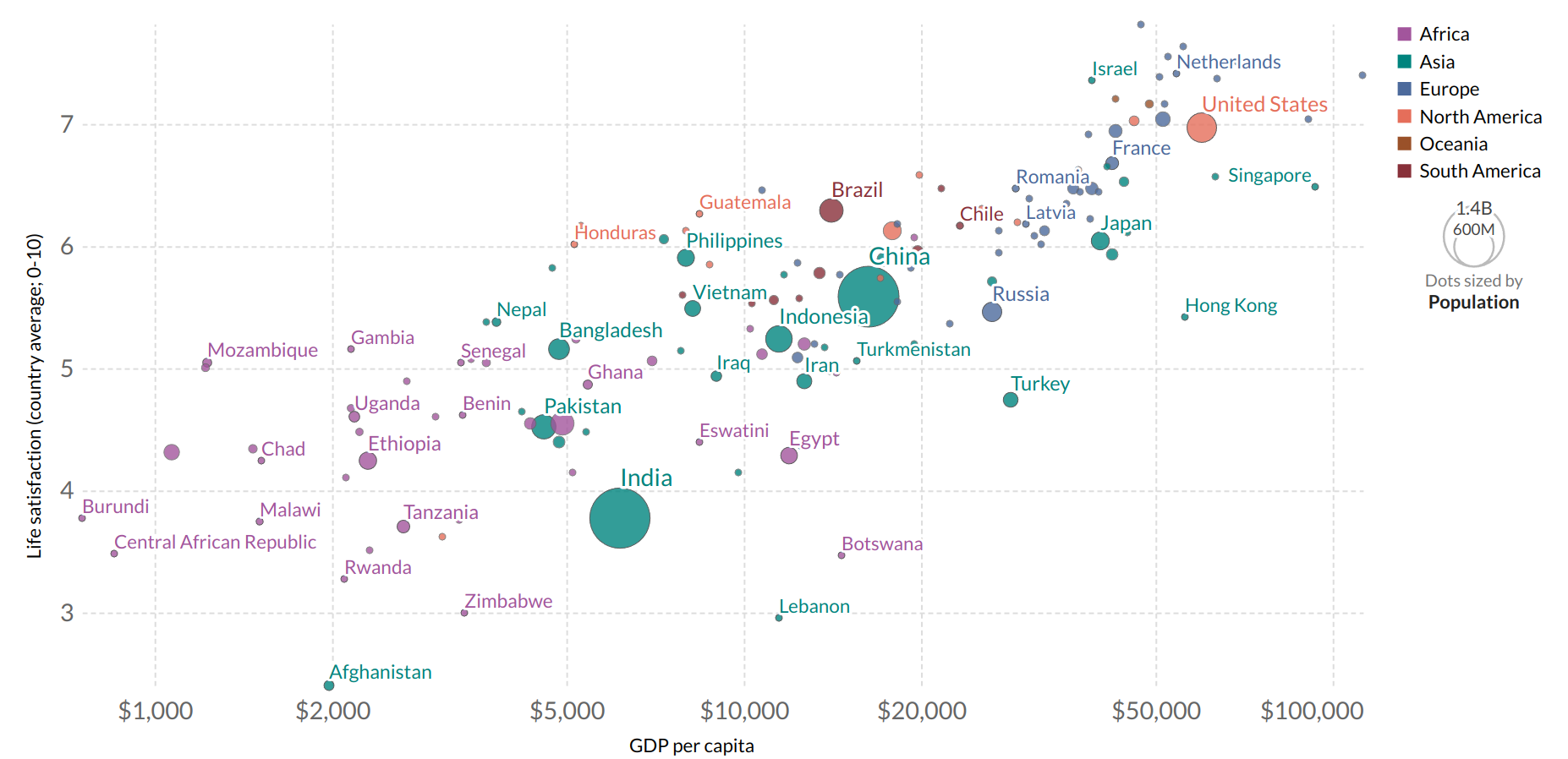
We do see a trend here. In the simplest scenario, we can model life satisfaction as a linear function of GDP per capita. This step is called model selection: we selected a linear model of life satisfaction with one attribute per capita.

life_satisfaction = $ \theta_{0} + \theta_{1} $ * GDP_per_capita

This model is simply a linear function of the input feature GDP_per_capita. This model has two parameters $ \theta_{0} + \theta_{1} $ which can be tweaked to represent any linear function. Our model makes a prediction by simply computing a weighted sum of the input features, plus a constant called bias term (also called intercept). Remember, we're doing supervised learning here, so that means we already have an idea about what the input/output cause and effect should be. Internally, the learner needs to learn the parameters $ \theta_0 $ and $ \theta_1 $. We can visualise what the effect of model is on tweaking these parameters:

theta_list = [(1, 2), (2,1), (1,0), (0,1)]
for theta0, theta1 in theta_list:
    x = np.arange(10)
    y = theta1 * x + theta0
    plt.plot(x,y)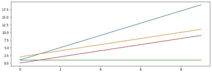

Model representation:

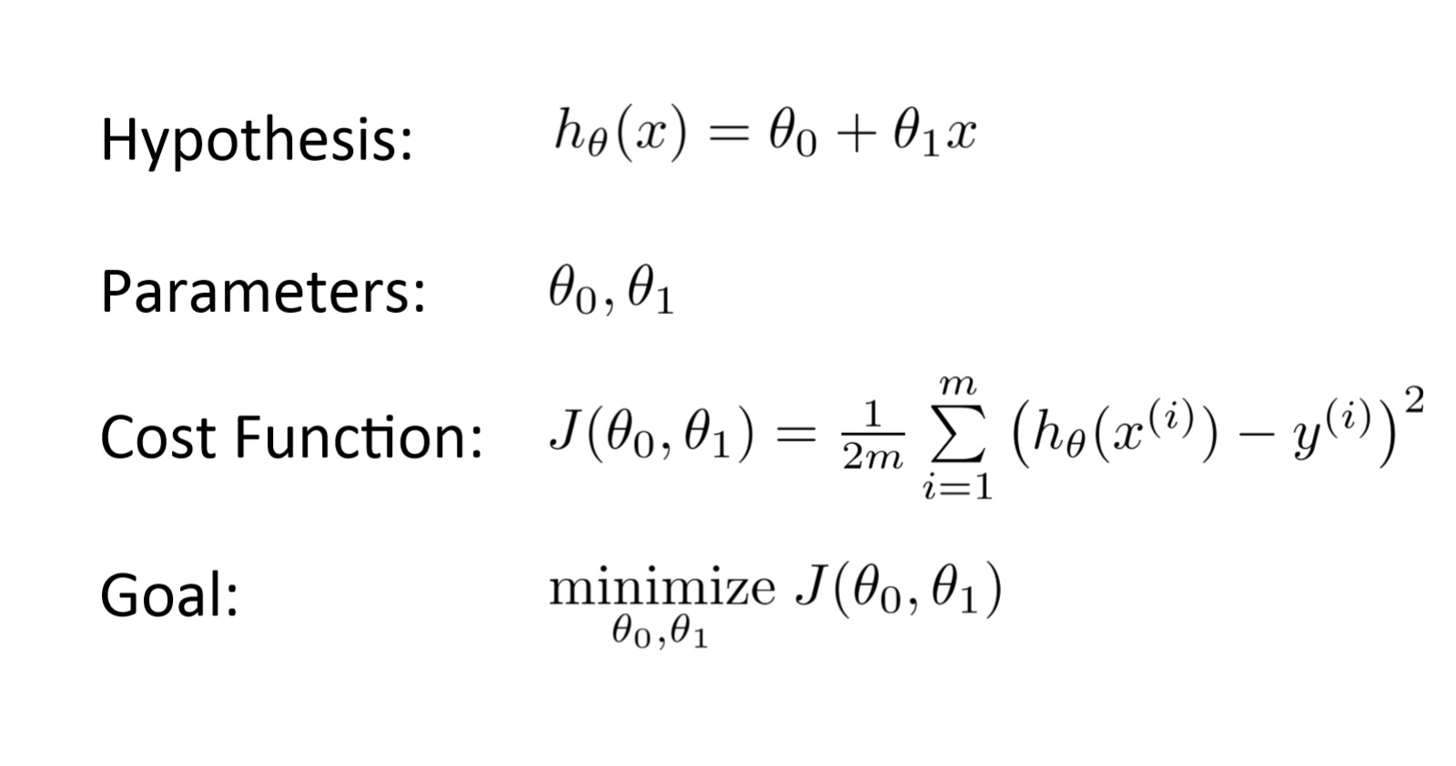
Given the training set, our goal is to construct a learner that will output a function donated by $ h $ (hypothesis), which takes as input $x_{1}, x_{2}, ...x{n} $ features and outputs an estimate Y. i.e learn $ h: X-> Y$ so that h(x) is a good predictor for the corresponding value of Y.

Formally, to perform supervised learning, we must decide how we're going to represent functions/hypotheses $ h $ in a computer. As an initial choice, let's say we decide to approximate $y$ as a linear function of $x$ :

$$‌‌h_{\theta}(x)=\theta_{0}+\theta_{1} x_{1}+\theta_{2} x_{2}‌‌+...+\theta_{n} x_{n}‌‌$$‌‌

Here, the $ \theta{i} $ 's are the parameters (also called weights) parameterizing the space of linear functions mapping from $ \mathcal{X} $ to $ \mathcal{Y} $.

$$‌‌\hat{y}=h_\theta(x)= \theta \cdot x‌‌ $$

In this equation:

$ \theta $ is the model's parameter vector, containing the bias term and the feature weights $ \theta_{1} $ to $ \theta_{n} $.
$ x $ is the instance's feature vector containing $ x_{0} $ to $ x_{n} $ , with $ x_{0} $ always equal to 1.
$ \theta \cdot x‌‌ $is the dot product of the vetor $ \theta $ and $ x $
$ h_\theta(x) $ is the hypothesis function, using the model parameters $ \theta $

Cost function:

Now, given a training set, how do we pick, or learn, the parameters $\theta$ ? We need to specify a performance measure that measures how good your model is or a cost function that measure how bad it is. One reasonable method seems to be to make $h(x)$ close to $y$, at least for the training examples we have. Formally, we can measure the accuracy of our hypothesis function by using a cost function.

$$‌‌J\left(\theta_0, \theta_1\right)=\frac{1}{2 m} \sum_{i=1}^m\left(h_\theta\left(x^{(i)}\right)-y^{(i)}\right)^2‌‌$$‌‌

Here we take difference between predicted value and actual value. This function is called mean squared error. The error metric provides a way to measure distance between two vectors (prediction vector and target values). This allows us to choose $ \theta_0 $ and $ \theta_1 $ so that $ h(\theta) $ is close to y for our training examples $ (x,y) $. Next our goal is to minimize this cost function:
$$
\underset{\theta_{0}, \theta_{1}}{\operatorname{minimize}} J\left(\theta_{0}, \theta_{1}\right)
$$

Training the Model:

Training a model means searching for a combination of model parameters that minimize a cost function. It is a search in the model's parameter space: the more parameters a model has, the more dimensions this space has and the harder the search is: searching for a needle in a 300-dimensional haystack is a much trickier than in 3 dimensions.

To make a machine learning algorithm, we need to design an algorithm that will improve the parameters (or weights $\boldsymbol{w}$) in a way that reduces MSE $_{\text {test }}$ when the algorithm is allowed to gain experience by observing a training set $ \left(\boldsymbol{X}^{(\text {train })}, \boldsymbol{y}^{(\text {train })}\right) . $

Minimize the mean squared error on the training set, MSE $_{\text {train }} .$ i.e $‌‌\underset{\theta_0, \theta_1}{\operatorname{minimize}} J\left(\theta_0, \theta_1\right) $

There are two ways to train this particular regression model. One is using a direct 'closed form' equation that directly computes the model parameters that best fit the model to the training set. The other method uses an iterative optimization approach called Gradient Descent that gradually tweaks the model parameters to minimize the cost function over the training set.

If we try to think of it in visual terms, our training data set is scattered on the $ x-y $ plane. We are trying to make straight line (defined by $ h_\theta(x) $ ) which passes through this scattered set of data. Our objective is to get the best possible line. The best possible line will be such so that the average squared vertical distances of the scattered points from the line will be the least. In the best case, the line should pass through all the points of our training data set. In such a case the value of $ J\left(\theta_0, \theta_1\right) $ will be 0. For this post we will focus on learning gradient descent as a method for finding the optimal model parameters.

Gradient Descent

Gradient Descent is a iterative optimization algorithm capable of finding optimal solutions to a wide range of machine learning problems. Gradient descent is an iterative approach for tweaking the model parameters to minimize the cost function over the training set.

Let's understand how works intuitively.

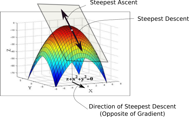
Suppose you are lost in the mountains in a dense fog, and you can only feel the slope of the ground below your feet. A good strategy to get to the bottom of the valley quickly is to go downhill in the direction of the steepest slope. This is exactly what Gradient Descent does: it measures the local gradient of the error function with regard to the parameter vector $ \theta $ and it goes in the direction of descending gradient. Once the gradient is zero, you have reached a minimum! Concretely, you start by filling (theta) with random values (also known as random initialisation). Then you improve it gradually, taking one baby step at a time, each step attempting to decrease the cost function (MSE) until the algorithm converges to a minimum.

Technical explanation:

Gradient descent can be used to find optimal parameters for linear and logistic regression, SVM and also neural networks which we consider later. The gradient descent algorithm can be utilized for the minimization of convex functions. Stationary points are required in order to minimize a convex function. A very simple approach for finding stationary points is to start at an arbitrary point, and move along the gradient at that point towards the next point, and repeat until converging to a stationary point. The way we do this is by taking the derivative (the tangential line to a function) of our cost function. The slope of the tangent is the derivative at that point and it will give us a direction to move towards. We make steps down the cost function in the direction with the steepest descent, and the size of each step is determined by the parameter $\alpha$, which is called the learning rate. i.e To find a local minimum of a function using gradient descent, one starts at some random point and takes steps proportional to the negative of the gradient (or approximate gradient) of the function at the current point.

The gradient descent algorithm is:

repeat until convergence:

$$‌‌\theta_j:=\theta_j-\alpha \frac{\partial}{\partial \theta_j} J\left(\theta_0, \theta_1\right)‌‌$$

where $ j=0,1 $ represents the feature index number.

Intuitively, this could be thought of as:

repeat until convergence:

$$‌‌\theta_j:=\theta_j-\alpha \text { [Slope of tangent aka derivative in } \mathrm{j} \text { dimension] }‌‌$$‌‌

‌

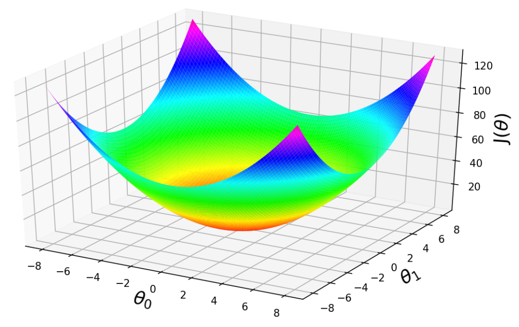
Imagine that we graph our hypothesis function based on its fields $\theta_0$ and $ \theta_1 $ (actually we are graphing the cost function as a function of the parameter estimates). We put $ \theta_0 $ on the $ x $ axis and $ \theta_1 $ on the $ y $ axis, with the cost function on the vertical $z$ axis. This can be kind of confusing. Essentially, we are moving up to a higher level of abstraction. We are not graphing $ x $ and $ y $ itself, but the parameter range of our hypothesis function and the cost resulting from selecting a particular set of parameters.

The points on our graph will be the result of the cost function using our hypothesis with those specific theta parameters. We will know that we have succeeded when our cost function is at the very bottom of the pits in our graph, i.e. when its value is the minimum.

Learning rate hyperparameter: An important parameter is Gradient Descent is the size of the steps, determined by the learning rate hyperparameter. If the learning rate is too small, then the algorithm will have to go through many iterations to converge, which will take a long time. On the other hand, if the learning rate it too high, you might jump across the valley and end up on the other side, possibly even higher up than you were before. Also note that not all cost functions look nice, regular bowls. There may be holes, ridges, plateaus, and all sorts of irregular terrains, making convergence to the minimum difficult.

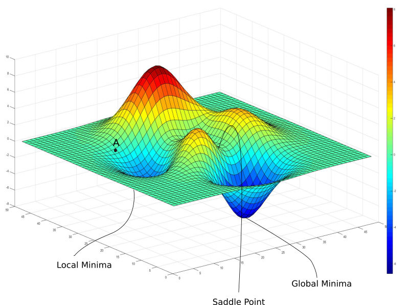
Fortunately, the MSE cost function for linear regression is a covex function. So this means there are no local minima, just one global minimum. If the features have different scales, it becomes a elongated scale. There many models, such as logistic regression or SVM, the optimization criterion is convex. Convex functions have only one minimum, which is global. Optimization criteria for neural networks are not convex, but in practice even finding a local minimum local minimum suffices.

When specifically applied to the case of linear regression, a new form of the gradient descent equation can be derived. We can substitute our actual cost function and our actual hypothesis function and modify the equation to:

repeat until convergence: {

$$‌‌\begin{aligned} \theta_0 & :=\theta_0-\alpha \frac{1}{m} \sum_{i=1}^m\left(h_\theta\left(x_i\right)-y_i\right) \\ \theta_1 & :=\theta_1-\alpha \frac{1}{m} \sum_{i=1}^m\left(\left(h_\theta\left(x_i\right)-y_i\right) x_i\right) \\ & \} \end{aligned}‌‌$$‌‌‌‌

To summarise the story so far, while implementing a supervised learning ML solution we have a dataset consists of training examples, which are pairs of inputs and targets. Each input is a vector of features or attributes. A learning algorithm can be fully defined by a model class, objective and optimizer. A cost/loss function measures the model performance or accuracy (the proportion of examples for which the model produces the correct output) or error rate (the proportion of examples for which the model produces an incorrect output). And finally an optimisation procedure like gradient descent is used for training the model.The output of a supervised learning is a predictive model that maps inputs to targets.

Components of a Supervised Machine Learning Problem

$ \underbrace{\text{Dataset}}_\text{Features, Attributes, Targets} + \underbrace{\text{Learning Algorithm}}_\text{Model Class + Objective + Optimizer } \to \text{Predictive Model} $

Example:

import numpy as np
from sklearn.kernel_ridge import KernelRidge

# We will load the dataset from the sklearn ML library

from sklearn import datasets
boston = datasets.load_boston()

# Apply a supervised learning algorithm

model = KernelRidge(alpha=1, kernel='poly')
model.fit(boston.data[:,[12]], boston.target.flatten())
predictions = model.predict(np.linspace(2, 35)[:, np.newaxis])

# Visualize the results

plt.scatter(boston.data[:,[12]], boston.target, alpha=0.25)
plt.plot(np.linspace(2, 35), predictions, c='red')
plt.ylabel("Median house price ($K)")
plt.xlabel("% of adults in neighborhood that don't have a high school diploma")
plt.title("House prices as a function of average neighborhood education level")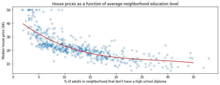

This concludes our introduction for supervised learning. This is one kind of machine learning where we had labelled data available. Unsupervised learning attempts to extract information from data without labels, e.g., clustering and density estimation. For example, Visualization algorithms like T-SNE are good examples of unsupervised algorithms, you feed them a lot of complex unlabelled data, and they output a 2D or 3D representation of your data that can easily be plotted. These algorithms try to preserve as much structure as they can so that we can understand how the data is organized and perhaps identify unsuspected patterns.

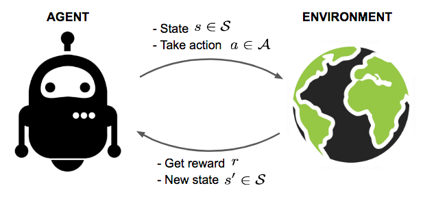
Lastly, Reinforcement learning is akin to optimal control, where the goal of the agent is to find the optimal sequence of actions that leads to the maximum reward. The agent acts in the world and receives feedback from the environment in the form of rewards or penalties based on its actions. The agent's goal is to learn a policy, or a mapping from states to actions, that maximizes the expected cumulative reward over time.