Array Programming with Numpy

Numpy is open source numeric and scientific computations library created around 2005. Numpy is also highly popular in scientific community and has recently been used to perform computations needed to discover black holes and gravitational waves. It provides a multidimensional Python array object (a data structure that efficiently stores and accesses tensors) along with array-aware functions that operate on it.

taken from https://www.nature.com/articles/s41586-020-2649-2.pdf

NumPy arrays:

Let's create a 5x5 array with random entries having type float64.

data = np.random.randn(5, 5)

array([[ 0.68658851, -0.8792515 ,  0.42941987, -0.4272763 ,  0.13740024],
       [-2.00408105,  1.54283662,  0.03151733,  1.40220172,  0.68258722],
       [-1.03817937, -0.06616036, -1.43253386,  0.0846872 , -0.43482168],
       [-1.09642464, -0.8237213 ,  0.48105926, -0.41901052,  0.74557661],
       [-0.19769946,  0.59291267, -0.39273076, -0.45374354,  0.79950827]])

We can also check their type

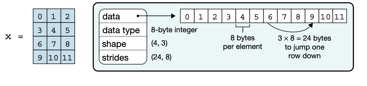
my_marray.shape,  my_marray.dtype

Numpy supports real and complex numbers (of lower and higher precision), strings, timestamps and pointers to Python objects and we can access elements using the index. The shape of an array determines the number of elements along each axis, and the number of axes is the dimensionality of the array. The data type describes the nature of elements stored in an array. An array has a single data type, and each element of an array occupies the same number of bytes in memory. Examples of data types include real and complex numbers (of lower and higher precision), strings, timestamps and pointers to Python objects[2].

Similarly we can create an identity matrix:

identity_matrix = np.identity(10, dtype = int)

output:


array([[1, 0, 0, 0, 0, 0, 0, 0, 0, 0],
       [0, 1, 0, 0, 0, 0, 0, 0, 0, 0],
       [0, 0, 1, 0, 0, 0, 0, 0, 0, 0],
       [0, 0, 0, 1, 0, 0, 0, 0, 0, 0],
       [0, 0, 0, 0, 1, 0, 0, 0, 0, 0],
       [0, 0, 0, 0, 0, 1, 0, 0, 0, 0],
       [0, 0, 0, 0, 0, 0, 1, 0, 0, 0],
       [0, 0, 0, 0, 0, 0, 0, 1, 0, 0],
       [0, 0, 0, 0, 0, 0, 0, 0, 1, 0],
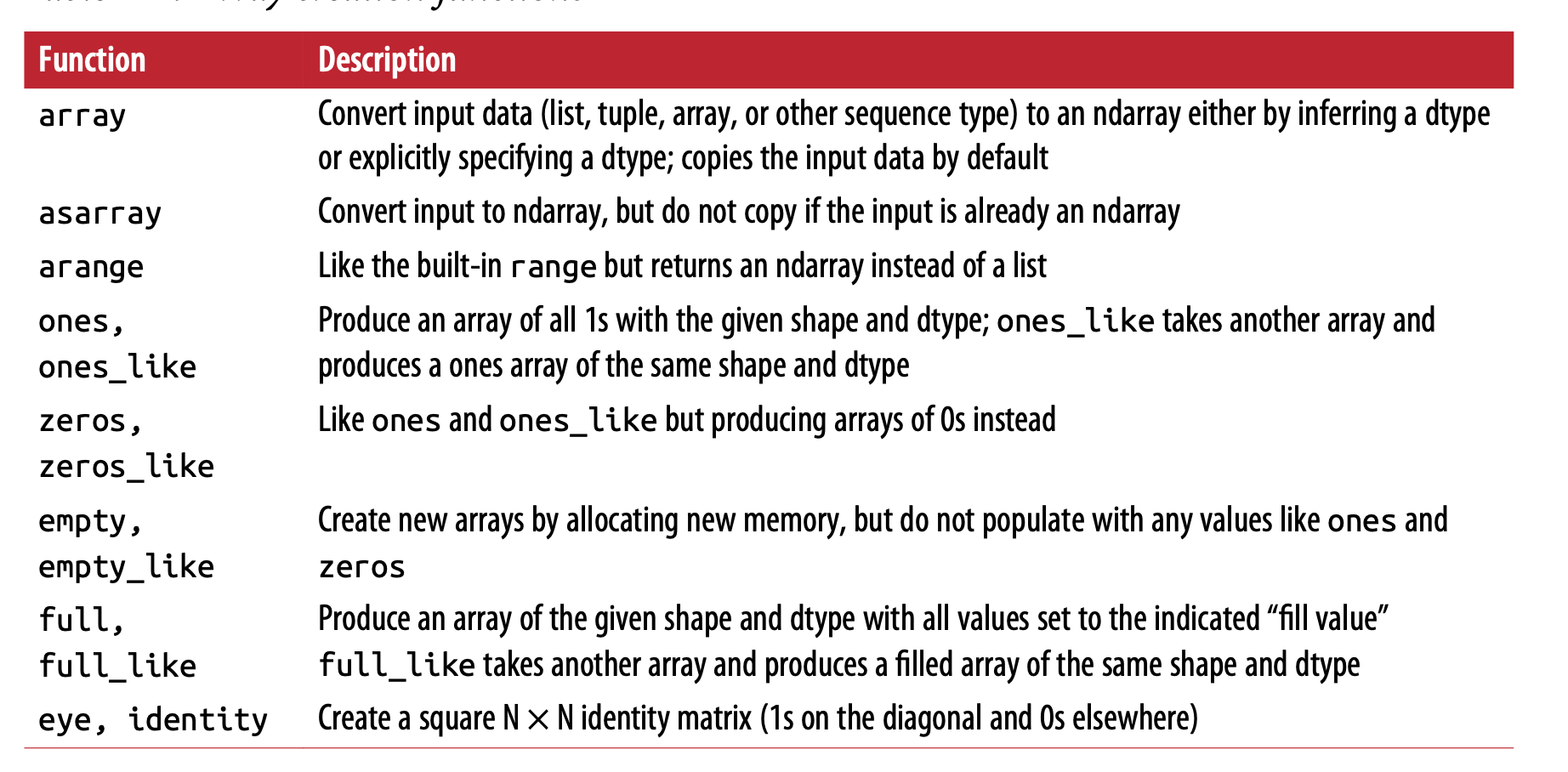
       [0, 0, 0, 0, 0, 0, 0, 0, 0, 1]])

We can create a numpy array using a number for methods. For example we can pass any sequence like python list to create a 1-dimensional array or nested lists to create multi-dimensional lists.

my_mdata = [[1, 2, 3, 4], [5, 6, 7, 8],[9,10,11,12]]

This creates a 3x3 matrix with entries having int datatype.

array([[ 1,  2,  3,  4],
       [ 5,  6,  7,  8],
       [ 9, 10, 11, 12]])

numpy provides many functions to create arrays (taken from [1])

Array indexing

We can interact with NumPy arrays using ‘indexing’. Array indexing is a rich topic and the general syntax is as follows:

X[start:end:step] #any of which can be left blank

These operations return a ‘view’ of the original data. To learn about it by trying some code:

my_mdata = np.array([[1, 2, 3, 4], [5, 6, 7, 8],[9,10,11,12]])

#select the first two rows of the multi-dimensional array
my_mdata[:2] 

#select first two rows and columns 1 onwards
my_mdata[:2,1:] 

#select third row
my_mdata[2,:]  

#again selects third row
my_mdata[2] 

#select row third onwards and all columns
my_mdata[2:,:] 

#all rows of third column
my_mdata[:,2] 

#all rows of first two columns
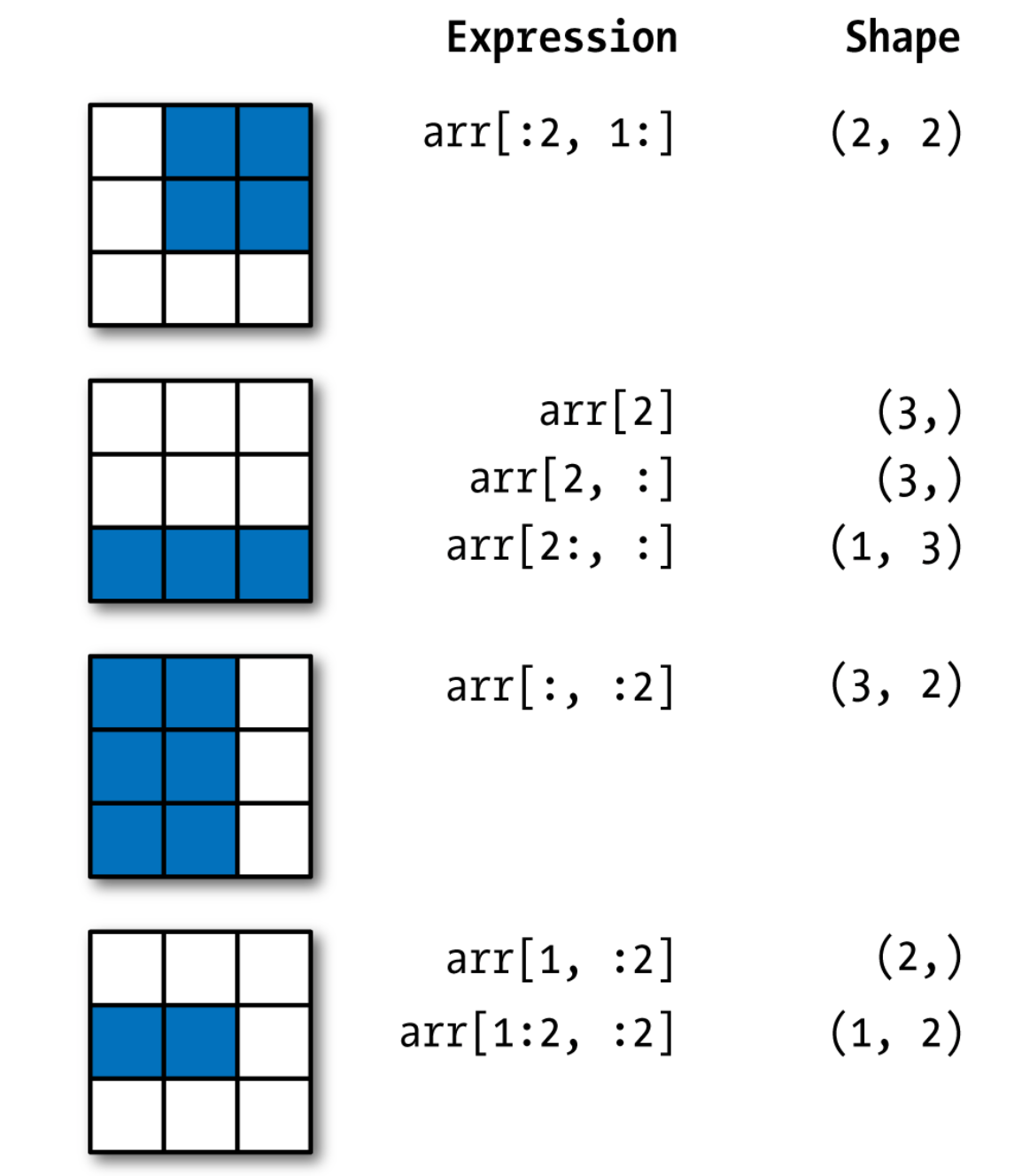
my_mdata[:,:2]

visualisation is the best way to understand the outputs:

*array slicing outputs (*taken from [1])

Fancy Indexing:

Arrays can even be indexed using other arrays.

Vectorization:

A key concept of array programming is Vectorisation. With vectorizaiton ability Numpy allows us to operate on entire arrays, rather than looping on individual elements like in C language. This leads to efficient code that can perform complex computations.

def myfunc(x):
    if x >=0:        
    	return True    
    else:       
    	return False print f(3)

f_vec = np.vectorize(f) #equavialent to above a single, clear Python expression

array-aware functions, such as sum, mean and maximum, perform element-by-element ‘reductions’, aggregating results across one, multiple or all axes of a single array

Linear Algebra:

import numpy as np

x = np.array([[1,2],[3,4]], dtype=np.float64)
y = np.array([[5,6],[7,8]], dtype=np.float64)

# Elementwise sum; both produce the array
# [[ 6.0  8.0]
#  [10.0 12.0]]
print(x + y)
print(np.add(x, y))

# Elementwise difference; both produce the array
# [[-4.0 -4.0]
#  [-4.0 -4.0]]
print(x - y)
print(np.subtract(x, y))

# Elementwise product; both produce the array
# [[ 5.0 12.0]
#  [21.0 32.0]]
print(x * y)
print(np.multiply(x, y))

# Elementwise division; both produce the array
# [[ 0.2         0.33333333]
#  [ 0.42857143  0.5       ]]
print(x / y)
print(np.divide(x, y))

# Elementwise square root; produces the array
# [[ 1.          1.41421356]
#  [ 1.73205081  2.        ]]
print(np.sqrt(x))

import numpy as np

x = np.array([[1,2],[3,4]])
y = np.array([[5,6],[7,8]])

v = np.array([9,10])
w = np.array([11, 12])

# Inner product of vectors; both produce 219
print(v.dot(w))
print(np.dot(v, w))

# Matrix / vector product; both produce the rank 1 array [29 67]
print(x.dot(v))
print(np.dot(x, v))

# Matrix / matrix product; both produce the rank 2 array
# [[19 22]
#  [43 50]]
print(x.dot(y))
print(np.dot(x, y))

Boolean array indexing:

Boolean array indexing lets you pick out arbitrary elements of an array. Frequently this type of indexing is used to select the elements of an array that satisfy some condition. Here is an example: